Lossy Image Compression
Every time you take a picture on your phone, most of the data is thrown away. Lossy image compression is the art of throwing away what your eyes won’t notice.
Note: at no point will this blog cover middle-out compression
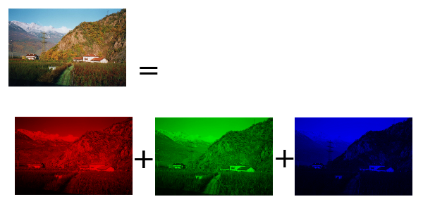
the pixels on most screens emit three different colors of light: red , green and blue . The reason those colors where chosen is that human color perception is enabled by cone cells, with cells that respond to red, green and blue light.
Human cone cells are sensitive to color, but rod cells are sensitive to brightness. And it turns out that rod cells are more sensitive, so humans can see changes in brightness with much higher resolution than changes in color. This is the first fact we will use to start compressing an image.
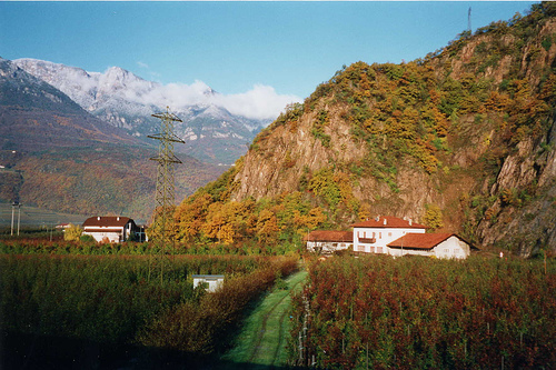
This will be our starting image:
This can be decomposed into R,G and B components:
What we want is a way to decompose the image into brightness and color components, that way we can use the fact that the eyes are more sensitive to brightness differences to compress this information. Specifically, we can shrink the color components since the eyes will have a hard time noticing.
There is a way to do this already, it’s called YUV color space. The Y is the brightness component, called the luma and the U,V components are the color components, collectively called the chroma.
The way to calculate the YUV values from the RGB values is given by these equations:
$$Y = k_r R + k_g G + k_b B $$ $$U = R - Y$$ $$V = B - Y$$
Since human eyes are less sensitive to the chroma (U and V), we can simply shrink each one by 1/2 along the width and height dimensions, that compresses it by a factor of four.
We can visualize it like this:
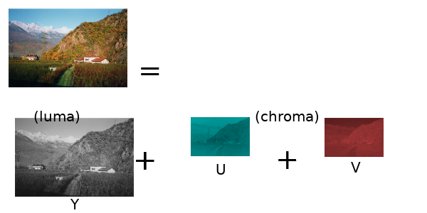
Then imagine we take U and V, and then scale them back up, they will have lost 3/4 of the original pixel values. With three components, and two scaled down to 1/4th, the total data left will be (1 + 1/4 + 1/4)/3 = 2 times smaller.
The actual color space used in JPEG and other common image compression algorithms is a variant of YUV called YCbCr, the equations are given in terms of RGB components:
$$Y = k_r R + k_g G + k_b B $$ $$C_b = \frac{(B - Y)}{2(1-k_b)} + 0.5$$ $$C_r = \frac{(R - Y)}{2(1-k_r)} + 0.5$$
The YCbCr color space is a standard defined by the ITU, or the International Telecommunications Union, which is currently an agency of the United Nations.
Throwing away the higher frequencies
This technique is not as obvious as the biologically inspired one above, but it’s brilliant, and once you see it, you cannot unsee it, this will change you forever.
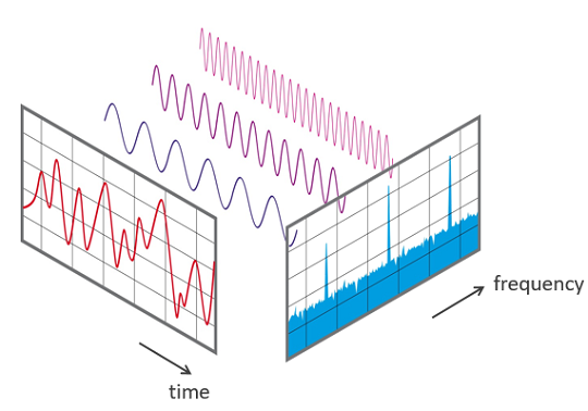
Imagine the red curve is a sound signal, vibrating over time. The Fourier transform calculates the blue chart showing the frequencies in the original signal. Those three perfect sine waves floating between those two charts represent the three highest peaks in the blue chart. They are the dominant frequencies in the red chart.
The above graphic came from Oleksii Trekhleb who has an excellent article explaining it in more detail. In this deep-dive, I want to focus on image compression, for that, we will need a transform that is related to Fourier, it’s called the Discrete Cosine Transform.
Instead of transforming a 1D signal in time, we want to transform a 2D signal in space, otherwise known as an image. Below I wrote an interactive transformer so you can see it in practice, then we can dive into the mathematics and start to understand how it works.
Click the pixels on the first square to see the discrete cosine transform on the second square. Click black dot to flip back to white. Try transforms of single black pixels, then try two pixels, turn pixels on and off to develop intuition to how the transformed image is constructed.
→After playing around with the transform for a while, you might notice that a single black dot usually transforms to a simple periodic image. The further to the bottom right you go, the higher frequency it transforms to.
Humans are much more sensitive to lower frequencies, so we can use this discrete cosine transform to throw away higher frequencies by deleting values in the lower right of the transformed image.
JPEG and other common image compression algorithms that use a DCT stage break the image into blocks of pixels called macroblocks, commonly sized at 8x8 or 16x16 pixels.
Call the macroblock $$M$$ and then define the following orthogonal matrix:
$$C_{mn} = k \cos\left( \frac{(2m+1)n\pi}{2N} \right)$$
Where $$k = \sqrt(1/N)$$ if n = 0, $$k = \sqrt(2/N)$$
otherwise. Finally, the DCT is the mapping $$M \to CMC^{-1}$$
Once we throw the higher frequencies away, there is not much else we can throw away that doesn’t start degrading the image quality, so we will turn to lossless compression, that is coming in the next post!